Comparative characterization of the infant gut microbiome and their maternal lineage by a multi-omics approach

Study design

We performed an intergenerational and observational study approved by the Regional Ethics Committee for Clinical Research of Hospital Universitario Infantil Niño Jesús in Madrid according to the ethical guidelines outlined in the Declaration of Helsinki and its amendments⁸⁷. The cohort of participants was initially recruited for a study regarding cow’s milk allergy, which showed scarce differences between allergic and non-allergic infants⁸⁸. Participants were recruited at Hospital Universitario Infantil Niño Jesús, Hospital General Universitario Gregorio Marañón and five Health Centers in Madrid (Spain). All participants provided informed consent.

Study population

The final study population consisted of 200 participants: 69 Infants up to twelve months of age, their 67 Mothers, and their 64 maternal Grandmothers. Infants were sex balanced, with a slightly higher proportion of females (55%) (Table S1). None of the infants had transitioned into a solid diet, and all were fed with either breastmilk alone, formula milk, or a combination of both. Mothers and grandmothers reported no dietary restrictions or specific diets. Exclusion criteria for all age groups were antibiotics intake in the 3 months prior to study recruitment and any other concomitant severe disease. Due to the difficulties in locating families with all three generations willing to participate, recruitment of the research population took two years.

All participating centers applied the same recruitment protocols and questionnaires. Information on age, sex, mode of birth, antibiotics use at birth, cow’s milk allergy and feeding regime for Infants, and age and smoking habits of Mothers and Grandmothers were collected. This data is presented in Supplementary Data 10, along with the family number and the techniques and datasets in which each sample was measured and/or included.

Sample collection and processing

Each participant received a sample collection kit developed by our group for easier collection at home. We published this procedure elsewhere^88,89. Subjects were asked to record the sample collection date, to not contaminate the sample with urine or toilet paper and to store the samples in the home freezer at −20 °C before taking them to the laboratory. A total of 200 fecal samples were collected at the laboratory and stored at −80 °C before being processed for metabolomics analysis and DNA extraction.

Gas chromatography coupled to QTOF mass spectrometry analysis (GC-QTOF-MS)

Prior to this study, we adapted a derivatization method that allows for shorter derivatization times <15 min³¹ compared to the 16 h of traditional approaches^32,35. It also enhances the coverage of key metabolites of the host-gut microbiota co-metabolism, such as SCFA, which have poor recoveries in the traditional derivatization reactions since they require anhydrous media and samples must be evaporated up to total dryness. We applied this methodology to a QTOF mass analyzer, a high-resolution equipment well-known for its powerful capabilities for unveiling unknown compounds. It allows for the determination of accurate mass in all detected mass-to-charge (m/z) fragments, which enormously enhances the selectivity and the sensitivity of the analysis and leads to a much more reliable identification^32,90. The samples analyzed were n = 67, n = 67, n = 63 of biologically independent samples for Infants, Mothers, and Grandmothers groups, respectively. The number of QCs were n = 24, and the biological replicates were n = 1.

Sample preparation

The protocol for sample preparation was adapted from Zhao et al.³¹, with some modifications⁴². Briefly, feces samples were lyophilized overnight at −110 °C in a LyoQest −85 lyophilizer (Telstar) until completely dried. Then, the lyophilizate from each individual sample was homogenized mechanically. Samples were taken as quickly as possible from the −80 °C freezer to avoid any thawing that would interfere with the lyophilization.

Metabolite extraction

10 mg of lyophilized feces were mixed with 300 μL of NaOH (1 M) solution in Milli-Q water and 10 μL of 1000 ppm 4-methyl valeric acid (4MV) solution, IS1, in a 0.5 mL Eppendorf tube and vortexed vigorously for 2 min. Samples were then centrifuged at 16,000 × g at 4 °C for 20 min. Each 200 μL of supernatant was transferred into an autosampler vial, and the residue was further extracted with 200 μL of cold methanol. After repeating the homogenization and centrifugation as above, 167 μL of supernatant was combined with the first supernatant in the sample vial. Blank samples were prepared in the same way, omitting the 10 mg of lyophilizate.

Derivatization with methylchloroformate (MCF)

To derivatize the extracted metabolites, 20 μL of MCF were added to each vial, as well as 34 μL of pyridine. The samples were then vortexed vigorously for exactly 30 s. Another 20 μL of MCF were added again, and samples were vortexed for another 30 s. Subsequently, 400 μL of 20 ppm tricosane (TRI) solution, IS2, in chloroform were added, and samples were vortexed for 30 s, followed by an addition of 400 μL of sodium bicarbonate solution (NaHCO₃, 50 mM in Milli-Q water) and additional vortexing for 30 s. Samples were then centrifuged at 2000 × g for 20 min at 4 °C in order to clearly visualize the double meniscus. Finally, 350 μL of the bottom chloroformic phase were transferred to transparent GC vials containing ∼100 mg of anhydrous sodium sulfate (Na₂SO₄).

GC-quadrupole-time of flight (QTOF)-MS equipment and analysis

The GC system (Agilent Technologies 7890B) consisted of an autosampler (Agilent Technologies 7693 A) and an Accurate-Mass Q-TOF (Agilent Technologies 7250). Data collection was performed with MassHunter Workstation GC/MS Data Acquisition Version 10.0. (Agilent).

GC-QTOF parameters were optimized from Zhao et al.³¹ to increase the coverage of relevant SCFAs by enabling the analysis of the most volatile SCFAs. One μL of each derivatized sample was injected using a splitless injection technique into a DB-5 MS capillary column (30 m × 0.25 mm i.d., 0.25 μm film thickness; (95% dimethyl/5% diphenyl) polysiloxane bonded and cross-linked with a precolumn (10 m) integrated; Agilent J&W Scientific, Folsom, CA), with helium as the carrier gas at a constant flow rate of approximately 1.0 mL·min⁻¹. The solvent delay time was set to 2.9 min. The optimized temperature gradient was the following: 30 °C held for 1 min, then increased at a rate of 10 °C·min⁻¹ up to 120 °C for 9 min, 20 °C·min⁻¹ to 320 °C for 10 min, and then held there for 2 min. The total time of analysis was 22 min. The temperatures of the injector, transfer interface, and ion source were set to 270, 270, and 220 °C, respectively. Electron impact ionization (70 eV) at the examined m/z range of 38 − 650 was used. The acquisition rate was 20 spectra·s⁻¹. To avoid signals from the solvents that could saturate the MS, the detector was turned off in the following retention time (RT) segments: 3.52–3.90 and 4.84–5.30.

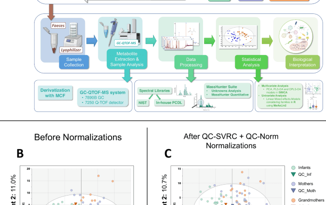
Experimental design for large-scale sample analysis in GC-QTOF-MS: batches and QC strategy

To be able to measure reliably all the samples from our cohort we divided them into three batches, according to the age group – batch 1: 67 Mothers, batch 2: 63 Grandmothers, and batch 3: 67 Infants. The samples were randomly measured inside their batch.

To later be able to join these batches and compare the data between them, we devised a quality control (QC) strategy. To prepare the QC samples, 17 mg of 30 lyophilized samples were taken (10 random samples from each of the 3 age groups) and a pool of 510 mg was obtained. This pool was split into three parts, one for each batch (170 mg per batch). Inside each batch, 11 QC samples were prepared, by taking 10 mg of the lyophilized feces and following the same protocol as the samples. From these 11 QCs, 3 were used as equilibrium QCs at the start of the analysis, and the other 8 were placed in the worklist every 9–10 samples – whose order was randomized inside each batch. This assured that the batches could be joined later by using a normalization strategy. Schematics detailing the preparation of QC samples and the worklists measured in the equipment are presented in Fig. S10.

Additionally, for GC-QTOF-MS a mix of n-alkanes was injected at the beginning of the worklist to later build calibration files that would allow converting RT into retention index (RI). This parameter is later used for the enhancement of metabolite annotation, as explained below.

Data treatment and compound identification in GC-QTOF-MS

The data treatment procedure was adapted from recently published protocols that have been rigorously tested and fine-tuned at CEMBIO³². GC-QTOF-MS data, peak detection, and spectra processing algorithms were applied using MassHunter Software (Agilent) using an untargeted workflow.

The overall analytical performance was carefully examined by inspection of total ion chromatograms (TIC) of experimental samples, QC samples, blanks, and both internal standards (IS): 4MV and TRI, following the guidelines of previous work on QA⁹¹. 4MV is the IS1 that is added before the derivatization and thus controls the reproducibility of the whole sample preparation process, while TRI is the IS2, added after the derivatization, and is used to control mostly the analytical performance of the GC-QTOF-MS equipment (drifts in response and performance of the injection process).

Then, the SureMass mass spectral deconvolution algorithm was applied in MassHunter Unknowns Analysis (B.10.0, Agilent) to identify co-eluted compounds by matching deconvoluted spectra and/or RTs to two spectral libraries: (i) a “Personal Compound Database and Library” (PCDL) built by analyzing chemical standards with the same method and (ii) a further search into the NIST20 library (National Institute of Standards and Technology, U.S. Department of Commerce). The details and parameters of these analyses are described in detail elsewhere³².

For obtaining the abundances of the metabolites, MassHunter Quantitative (B.10.0, Agilent) was used. First, the target ions were carefully checked with the experimental data, avoiding saturated ions and discarding compounds derived from the solvents, derivatizing agents or column bleeding. This process allowed the better revision of compound annotation using the NIST20 library with the tool MS Interpreter in NIST MS Search v.2.4 in MassHunter Qualitative (B.08.00, Agilent).

The result of the peak integration was an Excel file (Microsoft® Excel® for Microsoft 365 MSO v. 2401) for each batch (Infants, Mothers, and Grandmothers) (N = 161 features). The following step was a blank subtraction to ensure that signals from the reagents, solvents, contaminants, and derivatizing agents were removed (N = 152). Then, a quality assurance procedure (QA) was performed^92,93. First, we applied a filter by presence, where features that appeared in <50% of QCs and <70% of samples were removed (N = 152). Then, we applied a filter by Relative Standard Deviation (RSD), where metabolites were kept if they had, in at least one batch, an RSD < 30% in the QC samples (N = 134). This was performed independently for each batch.

Normalization procedures were also carried out to ensure the comparison between the three batches. First, an intra-batch correction using “QC Sample – Support Vector Regression Correction” (QC-SVRC)⁴³, and after the fusion of the three batches in a unique Excel, an inter-batch correction with QC-Norm^44,45 were applied. After these normalizations, the QA filters resulted in 152 features after the presence check and 146 final features after the RSD filter.

SCFA/BCFA and MUFA/PUFA ratios

The SCFA/BCFA ratio was calculated as the sum of the abundances of (Acetic + Propionic + Valeric + Caproic acid) divided by the sum of (Isotridecanoic acid + Isomyristic acid + Isopentadecanoic acid + Anteisopentadecanoic acid + [Iso/Anteiso]palmitic acid + Isomargaric Acid + Anteisomargaric acid).

The MUFA/PUFA ratio was calculated as the abundance of “Linoleic Acid/Oleic Acid” divided by the sum of (Arachidonic Acid + Eicosatrienoic Acid + Docosahexaenoic Acid). Both ratios were calculated from the data of GC-QTOF-MS for these metabolites.

Multivariate statistical analyses

After all the procedures described above, the data were imported into SIMCA (v.16.0.1, Sartorius Stedim Data Analytics AB) to build multivariate statistics models. Non-supervised models (PCA) and supervised models (PLS-DA and OPLS-DA) were obtained. The cross-validated scores from the OPLS-DA models and the “Variable Importance for the Projection” (VIP) values were also obtained from the significant models.

Multisegment injection (MSI) capillary electrophoresis coupled to TOF mass spectrometry analysis (MSI-CE-TOF-MS)

The samples were also measured in capillary electrophoresis coupled to MS (CE-MS), using a methodology published by Shanmuganathan and co-authors³⁸. This methodology, called Multisegment Injection (MSI)-CE-MS, is specially designed for large-scale studies, as in the present case, and employs serial injections of 13 samples in the CE system to allow for greater sample throughput (≈4 min/sample). In this case, we applied a targeted search for important metabolites of the gut microbiota metabolism that had not been previously detected in the GC-QTOF-MS analysis. The samples analyzed were n = 57, n = 66, n = 60 of biologically independent samples for Infants, Mothers, and Grandmothers groups, respectively. The number of QCs were n = 31, and the biological replicates were n = 1.

Sample preparation

We employed fecal extracts prepared by taking 25 mg of feces lyophilizate and extracting with a mixture of H₂O:ACN:IPA in a 10:6:5 (vol/vol/vol) proportion. This extract was filtered through Micro centrifuge filters (0.45 µm Nylon, Costar) at 16,100 × g for 15 min at 4 °C. For this extract to be suitable for MSI-CE-MS analysis, 100 μl aliquots of each sample were dried in a N₂ evaporator and reconstituted with 50 μl of H₂O:Methanol in a 70:30 proportion, containing the corresponding IS – 40 μM chloro-tyrosine (Cl-Tyr) as the IS for positive mode and 1 mM napthalene monosulfonic acid (NMS) as the IS for negative mode.

QC samples were prepared by pooling 5 μl of each sample in the study to a “Grand Pool”, from which six 50 μl aliquots were prepared by the same protocol as the rest of the samples. These QC samples were measured throughout the run to monitor analytical variability and equipment performance.

MSI-CE-TOF-MS equipment and analysis

Samples were measured in a G7100A CE equipment coupled to a 6230 TOF detector³⁸. The sample preparation and analysis in the equipment were performed in the Britz-McKibbin lab, at McMaster University (Hamilton, ON, Canada). Data collection was performed with MassHunter Workstation LC/MS Data Acquisition for 6200 series TOF (Agilent).

Targeted search of metabolites using in-house library

Once the data were obtained, they were processed following the published procedures³⁸. The QA procedures and statistical analyses were applied in the same way as for the GC-QTOF-MS data. Of note, GABA was not detected in all samples (total n = 160) due to isomeric interferences. Thus, a K-nearest neighbors (KNN) missing value imputation was carried out with a MATLAB script⁹⁴.

16S rRNA gene sequencing and shotgun metagenomic sequencing

For both genomic techniques – 16S rRNA gene sequencing and shotgun metagenomics – a subset of samples was selected, due to limitations in sample quantity. Therefore, 40 Infants, 45 Mothers, and 43 Grandmothers (n = 128) were included.

DNA extraction

DNA was extracted from 200 mg of feces using the QIAamp DNA Stool Mini Kit (QIAGEN, Hilden, Germany) following the manufacturer’s instructions plus an additional membrane disruption step using metal beads⁹⁵. The extracted DNA was quantified by Qubit® 2.0 Fluorometer following the dsDNA HS Assay Kit protocol. All 128 samples had a concentration higher than 0.2 µg/µL and were suitable for sequencing.

16S rRNA gene amplification and sequencing

The V3-V4 regions of the 16S rRNA gene were amplified and sequenced using the MiSeq platform from Illumina, as described in the manual for “16S Metagenomic Sequencing Library Preparation” of the MiSeq platform (Illumina, San Diego, California, EEUU).

Bioinformatics and statistical analyses for 16S rRNA gene sequencing

16S rRNA sequences were denoised and processed with DADA2 v1.11 in order to define ASVs⁹⁶. In addition, DADA2 and the command removeBimeraDenovo were used to remove chimeras. Taxonomy was assigned using the DADA2 implementation of the RDP classifier⁹⁷, using the formatted RDP training set 16 release 11.5 from the DADA2 website. Shannon’s α-diversity index was estimated using the package vegan v2.6-4 and the R 4.2.2 software. Richness was defined as the number of ASVs identified in a given sample.

For the cladogram of differences in species abundance between groups, we applied the linear discriminant analysis (LDA) effect size (LEfSe) tool⁹⁸, via the interactive webpage (https://huttenhower.sph.harvard.edu/galaxy/). This high-dimensional data analysis tool for biological indicators compares various groups, focuses on biological correlations and statistical significance, and identifies biological indicators that differ significantly between groups.

Shotgun metagenomics sequencing

Metagenomic sequencing was performed using a NextSeq platform (Illumina, USA) according to the manufacturer’s recommendations for obtaining paired-end sequences of 150 base pairs.

16S rRNA gene and shotgun sequencing phylum taxonomy

For both 16S rRNA gene sequencing and shotgun metagenomics sequencing, the phylum nomenclature was established using up to two nomenclature codes: previous informal names, and the new names published by the International Code of Nomenclature of Prokaryotes (ICNP)⁹⁹.

Bioinformatics and statistical analyses for shotgun metagenomics sequencing

First, the paired-end Fastq files were filtered by quality with the Fastp application (version 0.20.1)¹⁰⁰: low-quality bases were trimmed from the tail of each read, low complex reads were removed, and reads shorter than 35 bases were discarded. Next, all the reads passing the previous filters were mapped onto the Homo sapiens genome (GCA_000001405.28 GRCh38.p13 assembly) by means of Bowtie2 (version 2.4.2)¹⁰¹. Finally, the reads which did not align concordantly against the Homo sapiens genome were analyzed with the SqueezeMeta pipeline with coassembly mode (version 1.3.1; database built on September 2020)¹⁰². Tabular outputs were generated from the SqueezeMeta results using the sqm2tables.py SqueezeMeta script, ignoring unclassified reads in the TPM calculation.

Next, for shotgun sequencing data, we analyzed both taxonomic data (phyla, genera, and species) and metabolic functions. For functional pathways, we tested these differences at several levels: KEGG Orthology (KO) terms, that identify orthologous groups of genes organized using the BRITE functional hierarchy¹⁰³, and level B and C of the hierarchy, explained below.

We joined these KO terms according to the BRITE functional hierarchies (see https://www.genome.jp/kegg/kegg3b.html) to which they belong, obtaining: 52 BRITE functional hierarchies (level B), (e.g., Amino acid metabolism, Carbohydrate metabolism, Endocrine system), and 483 BRITE functional hierarchies (level C), (e.g., Histidine metabolism, Galactose metabolism, Glucagon signaling pathway).

For KEGG and BRITE the following parameters were used: minimum abundance and prevalence applied were: 0.0. The normalization was performed with the trimmed mean of M values method (TMM) also using a linear model test (LM) with a maximum significance 0.10.

Statistical univariate analysis

Analysis was performed using the MaAsLin2 (Microbiome Multivariable Associations with Linear Models) R package¹⁰⁴ applying GLM models establishing the family as the random effect and the generation as the fixed effect (Infants, Mothers, and Grandmothers). The False Discovery Rate (FDR) was performed, and statistical significance was set at 95% level (FDR < 0.05). We applied this test for the metabolomics data (GC-QTOF-MS and MSI-CE-MS), the taxonomic data from metagenomics (16S rRNA gene and shotgun sequencing) i.e. phyla, genera, and species, and the functional data from shotgun sequencing (KEGG and BRITE B and C functional hierarchies).

The MetaboAnalyst online tool (v. 6.0) was used for metabolomic pathway analysis. GraphPad Prism (v.9.5.0) was used to represent statistical graphs.

Multi-omics dataset integration using mixOmics

Integration of the different Omic datasets was performed with the mixOmics script⁴⁶ using the Data Integration Analysis for Biomarker discovery using Latent Components (DIABLO) framework⁴⁷ using R (v. 4.2.2). This is a multi-omics integrative method that seeks common information across different data types through the selection of a subset of molecular features, while discriminating between multiple phenotypic groups. For this integration we used the 113 samples that were common to all techniques used (Fig. S1B, Supplementary Data 10). We assessed the performance of the model using 5-fold cross-validation repeated 10 times with the function perf(). We then assessed the accuracy of the prediction on the left-out samples (KOs, ASVs, metabolites). ROC curves and AUC plots per block were plotted using the function auroc(). We set the number of variables to select to 25 on each of the 3 components (KOs, ASVs, Metabolites) of PLS-DA. The circosPlot was built based on a similarity matrix. A cutoff of 0.65 was included to visualize correlation coefficients above this threshold in the multi-omics signature.

Reporting summary

Further information on research design is available in the Nature Portfolio Reporting Summary linked to this article.